OrthoVenn Plus User Manual
Platform: OrthoVenn Plus · Online platform for multi-species comparative genomics
URL: https://orthovenn.com
Intended for: Researchers who need to perform multi-species comparative genomics, with no programming or command-line experience required.
Table of Contents
- Platform Overview
- Data Preparation & Format Requirements
- Analysis Workflow at a Glance
- Step 1: Select Species & Upload Data
- Step 2: Configure Analysis Modules
- Step 3: Preview & Submit
- Tracking Progress & Task History
- Interpreting & Exporting Results
- Positive Selection Analysis on Gene Clusters (run on demand after results are generated)
- Online Helper Tools (Web Tools)
- Local Deployment (Docker)
- FAQ & Troubleshooting
1. Platform Overview
OrthoVenn Plus integrates the many algorithms used in comparative genomics — which would otherwise have to be installed separately and chained together by hand — into a single, complete online workflow. You simply pick your species on the web page, set a few key parameters, and click submit to run the entire chain, from orthologous gene identification all the way to positive selection detection.
Scientific questions OrthoVenn Plus helps you answer:
- Which genes does my species share with its relatives, and which are unique to it?
- What is the evolutionary relationship among these species, and roughly when did they diverge?
- Which gene families underwent significant expansion or contraction during evolution?
- Did any genes experience positive selection (adaptive evolution) along particular lineages?
- Do the genomes of different species remain collinear at the chromosomal level?
The six analyses and how they relate to one another:
【Insert figure here: six-module workflow / technical roadmap diagram】
| Analysis | Purpose | Input | Main Output | How it runs |
|---|---|---|---|---|
| ① Orthologous cluster analysis | Group genes across species, extract single-copy orthologs, functional annotation | Protein sequences | Gene clusters, pan-genome structure, single-copy gene set, GO annotation | Required, runs with the task |
| ② Species tree analysis | Build the species phylogeny | Single-copy genes from ① | Species tree with support values | Runs with the task |
| ③ Divergence time estimation | Estimate absolute divergence ages | Species tree from ② + fossil calibration points | Time-calibrated tree | Runs with the task |
| ④ Gene family expansion & contraction | Detect significantly expanded/contracted gene families | Time tree from ③ + gene counts from ① | Expansion/contraction events on each branch | Runs with the task |
| ⑤ Chromosomal collinearity analysis | Detect conservation of chromosomal structure | GFF annotation | Collinear blocks, Sankey diagram | Runs with the task |
| ⑥ Positive selection analysis | Detect genes that underwent adaptive evolution | Gene cluster + CDS sequences | Positively selected branches/sites | Run on demand on the clusters of interest after results are generated (see Chapter 9) |
Why is positive selection "run on demand"? The first five analyses run automatically over the whole dataset, whereas positive selection targets one cluster of interest at a time (e.g. a family that expanded significantly). It requires you to first see the results and then choose which cluster to analyze, so it is not part of the submission wizard — instead it is triggered per cluster on the results page.
Built-in species database: The platform ships with a built-in database covering six major groups — vertebrates, invertebrates (metazoa), protists, fungi, plants and bacteria — comprising 1,566 species and roughly 19.7 million protein sequences (data source: Ensembl, 2025). All sequences have been format-unified, de-duplicated and ID-standardized. You can start an analysis simply by selecting species in the interface, with no need to download or prepare data yourself.
2. Data Preparation & Format Requirements
2.1 The Three Input File Types
| File type | Format | Purpose | When needed |
|---|---|---|---|
| Protein sequences | FASTA (.fa / .fasta) | Core input for orthologous cluster analysis | Required (basis for all analyses) |
| Gene annotation | GFF3 (.gff / .gff3) or BED (.bed) | Provides gene positions on chromosomes | Chromosomal collinearity analysis |
| CDS nucleotide sequences | FASTA (.cds.fa) | Provides codon-level information (dN/dS) | Positive selection analysis on gene clusters |
Protein sequences are the only required file. GFF and CDS are both optional — they are used only if you need collinearity or positive selection. You can either provide them together when you upload a species, or add them later (adding them later unlocks only the corresponding analysis and does not affect results already completed).
For species chosen from the built-in database, all three file types are already prepared — no upload is needed at all.
2.2 The Single Most Important Rule: Gene IDs Must Match Across the Three Files
This is the number-one cause of upload/analysis failure, so please read it first.
Within one species, the protein FASTA, CDS and GFF files must use the exact same ID to refer to the same gene:
Protein FASTA  >GeneA001   MSTDVPAK...
CDS  FASTA     >GeneA001   ATGTCTACT...
GFF  annotation  ... gene_id "GeneA001" ...
- If the CDS ID does not match the protein → positive selection cannot map the protein to its codons, and that cluster is flagged as not analyzable.
- If the GFF ID does not match the protein → the collinearity plot is empty or fails to render.
- The platform does not guess this correspondence from string similarity, so please confirm ID consistency before uploading (you can validate it in one click with the preprocessing tool in Chapter 10).
2.3 Protein FASTA Format
>GeneA001
MSTDVPAKTSVILGQITTADTCLDPAGRKVIYLSE...
>GeneA002
MKWVTFISLLFLFSSAYSRGVFRRDAHKSEVAHRFK...
Notes:
- Each sequence ID (the name after
>) must be unique within each species file. - Keep IDs concise and avoid spaces, slashes
/, and quotes' "and other special characters. - Use a different file name for each species; we recommend naming files after the full Latin species name (e.g.
Arabidopsis_thaliana.fa,Oryza_sativa.fa). The file name is used as the species name shown in the results, so please use meaningful names.
2.4 CDS Nucleotide Sequence Format
- The gene ID must be exactly identical to the ID in the corresponding protein FASTA (see 2.2).
- Sequences should ideally be complete codons (length a multiple of 3); if not, the platform handles it automatically — no manual padding required.
2.5 GFF / BED Annotation Format
- Must contain gene position information: chromosome, gene ID, start, end, strand.
- The gene ID must match the ID in the protein FASTA (see 2.2).
- Supports
.gff,.gff3,.bed. Standard GFF3 downloaded from Ensembl / NCBI / Phytozome can be converted in one click with the GFF to BED tool in Chapter 10. - Requirement specific to collinearity analysis: be sure to use chromosome-level annotation, and keep the number of distinct chromosomes below 50. If your annotation is at the scaffold/contig level (many fragments), please keep only the 50 longest fragments before uploading, otherwise the collinearity plot becomes hard to read (see 5.5).
2.6 Data Preprocessing Tools (strongly recommended)
Before uploading, we recommend checking your input files with the online helper tools under the TOOLS menu. They can automatically:
- detect and report duplicate sequence IDs;
- remove illegal characters and unify line breaks;
- convert GFF3 into the BED format the platform requires;
- validate ID consistency across the protein / CDS / GFF files.
A downloadable local version (Windows / macOS / Linux) is also available on the Resources page of the homepage.
3. Analysis Workflow at a Glance
The whole analysis runs in three steps, plus one optional on-demand analysis:
Step 1 Select species / upload data    Step 2 Configure modules        Step 3 Preview & submit
   ├ Built-in or upload proteins  ──▶   ├ Module 1 Orthology (required) ──▶  Runs in the background
   └ Optional: GFF / CDS               ├ Modules 2–5 toggle as needed       Email notification on completion
                                       └ Just set the Basic parameters

                          ────────  After results are generated  ────────▶
                          Chapter 9: run positive selection on demand for the clusters of interest
Parameters for each module are shown in two layers:
- Basic (expanded by default): the 2–4 key parameters that genuinely require a decision from you.
- Advanced (collapsed by default): tuning parameters that affect accuracy or runtime; the defaults are fine in the vast majority of cases.
About threads: the Advanced section of each module has a thread-count parameter, which is fixed at 48 and not editable in the online version (the platform schedules resources centrally). To customize threads and accelerate large-scale analyses, download the local deployment (see Chapter 11). Hovering over the parameter shows a download hint.
3.1 Parameter Changes & Versioned Reruns: Old Results Are Never Overwritten (OrthoVenn Plus signature feature)
The OrthoVenn Plus backend has been redesigned so that rerunning an analysis never overwrites the old results — a hallmark of this version that lets you explore the effect of different parameters quickly and efficiently.
Whenever you change a parameter that affects the computed result, the platform generates a new version of the affected module while keeping the old version for comparison; changes that only affect display (thresholds, colors, sorting, window size, etc.) merely refresh the view instantly and trigger no recomputation.
| Your change | Typical effect | Rerun needed? |
|---|---|---|
| GO p-value filter, table sorting, plot colors | Display only | No (instant view refresh) |
| Orthologous cluster algorithm or threshold | Affects orthogroups and almost all downstream | Rerun this module + all downstream |
| Species tree method or rooting | Affects time tree and CAFE5 | Rerun species tree and its downstream |
| Divergence time calibration points / Root Age | Affects time tree and CAFE5 | Rerun time tree and CAFE5 |
| CAFE5 k value | Affects expansion/contraction only | Rerun CAFE5 only |
| Positive selection method or foreground branches | Affects only the positive selection result of the chosen cluster | Rerun only the corresponding positive selection task |
| Collinearity display window size | View only | Usually no rerun |
Benefits of this design:
- Nothing is lost, everything is comparable: old results are always kept, so you can compare results from different parameters side by side (e.g. Inflation 1.5 vs 1.2, CAFE5 k=2 vs Base, different tree-building methods) and pick the most reasonable one.
- Compute only what's needed, save time and resources: the platform reruns only the affected module and its downstream; unaffected upstream results are reused automatically, with no need to start over.
- Fully reproducible: every result version is bound to three things — input data + normalized parameters + tool versions — so anyone can reproduce it exactly.
- Zero wait for display tweaks: changes that only affect the view (thresholds, colors, sorting, windows) take effect instantly and consume no compute.
Tip: on the results page you can see a version list for each module; switch versions to compare results under different parameters.
4. Step 1: Select Species & Upload Data
4.1 Steps
- Open OrthoVenn Plus, click Create to start a new project, and enter Step 1 · Species.
- Choose your data source:
Option A · Select from the built-in database (Cloud Species)- Type the Latin species name in the search box (fuzzy search supported) and click to add it to the analysis list.
- No files to upload; the sequences are already standardized.
Option B · Upload custom data (Custom Upload)- Drag your protein FASTA into the upload area, or click to choose files; multiple species can be uploaded at once (up to 12 species in the online version).
- Optional: if you plan to do collinearity or positive selection later, you can upload the corresponding GFF / CDS here as well; you can also add them later.
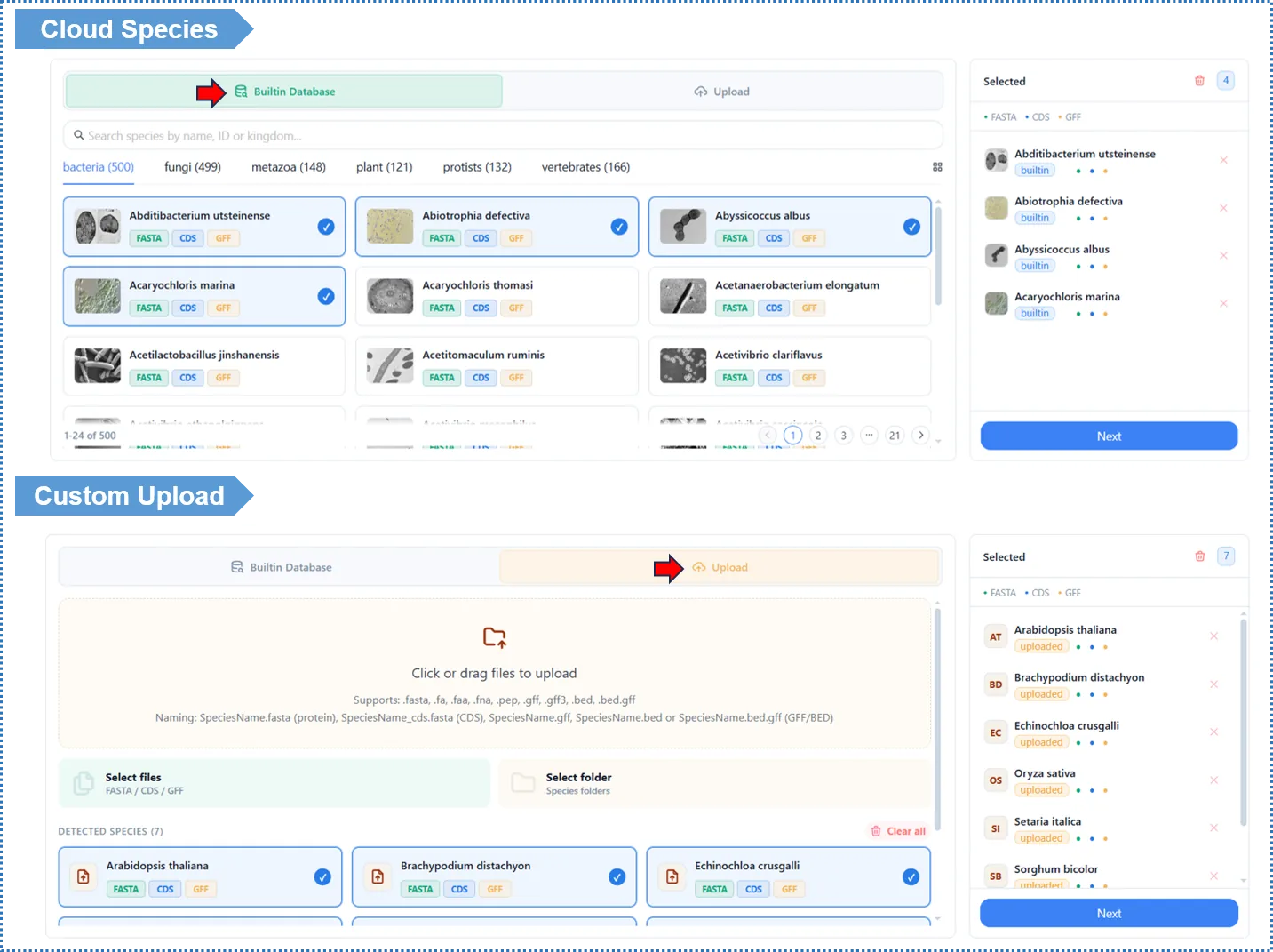
- The Added Species panel on the right lists the species you have added and the status of their files (protein / GFF / CDS). Please confirm the count and file types are correct.
- To practice first, click Load Example to load sample data.
- When everything looks right, click Next to go to Step 2.
4.2 Notes
- The two options can be combined: you can both select built-in species and upload custom species.
- GFF / CDS are optional; leaving them out does not affect core analyses such as orthology and the species tree.
- If a file has a format error, the platform flags it during upload.
- Compare within the same major group. Built-in species are intended to be compared within the same major group (e.g. plants with plants, fungi with fungi). Cross-kingdom comparisons (e.g. plants vs. bacteria) rarely yield biologically meaningful results, so the interface restricts built-in selection to a single group by default. If you genuinely need a cross-group comparison, prepare the species via custom upload.
5. Step 2: Configure Analysis Modules
The list of analysis modules is on the left. Module 1 (Orthologous cluster analysis) is required; Modules 2–5 can be toggled as needed. Click a module name to switch the parameter panel on the right.
Module dependencies (enabling a downstream module automatically includes its dependencies):
Module 1 (Orthology) ──▶ Module 2 (Species tree) ──▶ Module 3 (Divergence time) ──▶ Module 4 (Gene families)
Module 5 (Collinearity) is independent and only needs GFF
Tip: positive selection is not configured here. It is run on demand for individual clusters on the results page after results are generated (see Chapter 9).
5.1 Module 1 · Orthologous Cluster Analysis (required)
What does this module do for you?
It is the starting point of the whole workflow: it compares the proteins of all species pairwise and groups them into "clusters" (orthogroups) by similarity. Genes within the same cluster are considered to derive from a common ancestor. Outputs:
- Pan-genome structure: which clusters are shared by all species (the core genome) and which are unique to certain species.
- Single-copy orthologs: the set of genes present in exactly one copy in every species — the ideal data for building a species tree.
- GO functional annotation: the functional classification of each cluster, to help you understand its biological meaning.
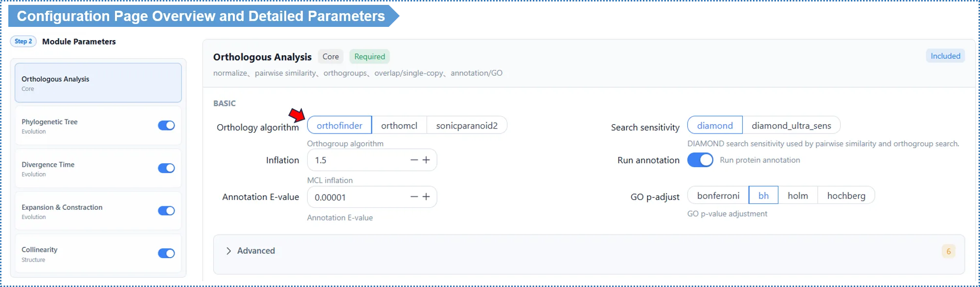
Basic Parameters
Orthology algorithm (Algorithm) — default OrthoFinder
| Algorithm | Characteristics | Use case |
|---|---|---|
| OrthoFinder (recommended, default) | Based on gene-tree/species-tree reconciliation; distinguishes orthologs (from speciation) from paralogs (from gene duplication); high accuracy | Most comparative genomics analyses |
| OrthoMCL (classic) | The classic method based on global sequence-similarity + Markov clustering (MCL), with cluster granularity controlled by the Inflation value | General use, moderate evolutionary distance; when you need to compare against classic OrthoMCL-based literature |
| SonicParanoid2 (advanced) | An ultra-fast algorithm optimized for large datasets | Many species (>30) or rapid exploration |
How to choose? If unsure, use OrthoFinder — currently the most accurate and general-purpose method, and the only one that explicitly distinguishes orthologs from paralogs. If you want the classic MCL clustering approach, or need to compare against existing OrthoMCL results, choose OrthoMCL (note it is more sensitive to the Inflation value, see below). Only consider SonicParanoid2 when you have many species and want a quick first pass.
Search Sensitivity — default Standard (diamond)
- Standard (fast): suitable for most cases and quick.
- Ultra-sensitive (diamond_ultra_sens, slow): finds more distant homology, suitable for evolutionarily distant species (e.g. cross-phylum comparisons), but slower.
How to choose? Standard is fine for closely related species; choose ultra-sensitive when the species are distant and you are worried about missing distant homologs.
Inflation value (MCL clustering tightness) — default 1.5
- Used for MCL-based clustering (OrthoMCL, and the MCL step inside OrthoFinder). It controls cluster "tightness": higher values give smaller, tighter clusters; lower values give larger, looser ones.
- How to choose? Keep 1.5 in most cases. If clearly related genes are being split into different clusters, lower it to 1.2; if a single cluster mixes functionally divergent genes, raise it to 2.0. The effect is more pronounced when OrthoMCL is selected.
Functional annotation (Run Annotation) — default on
- When on, it produces GO functional annotation and enrichment analysis. We strongly recommend keeping it on as the basis for downstream functional interpretation; turn it off only to save time.
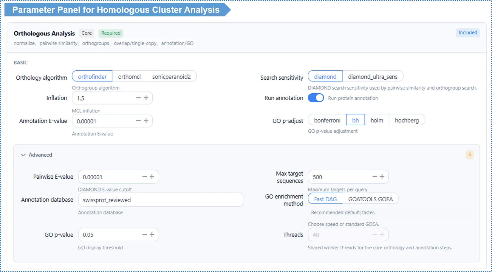
Advanced Parameters
| Parameter | Default | Description |
|---|---|---|
| Alignment E-value | 1e-5 | Statistical significance threshold for homology calls. Looser (1e-2) suits distant species; stricter (1e-10) suits fine-grained comparison of close relatives. Rarely needs changing |
| Annotation database | Swiss-Prot reviewed | Reference database for functional annotation |
| GO multiple-testing correction | BH (FDR) | p-value correction method for enrichment analysis |
| Threads | 48 | Read-only online; editable locally |
Interpreting the Results
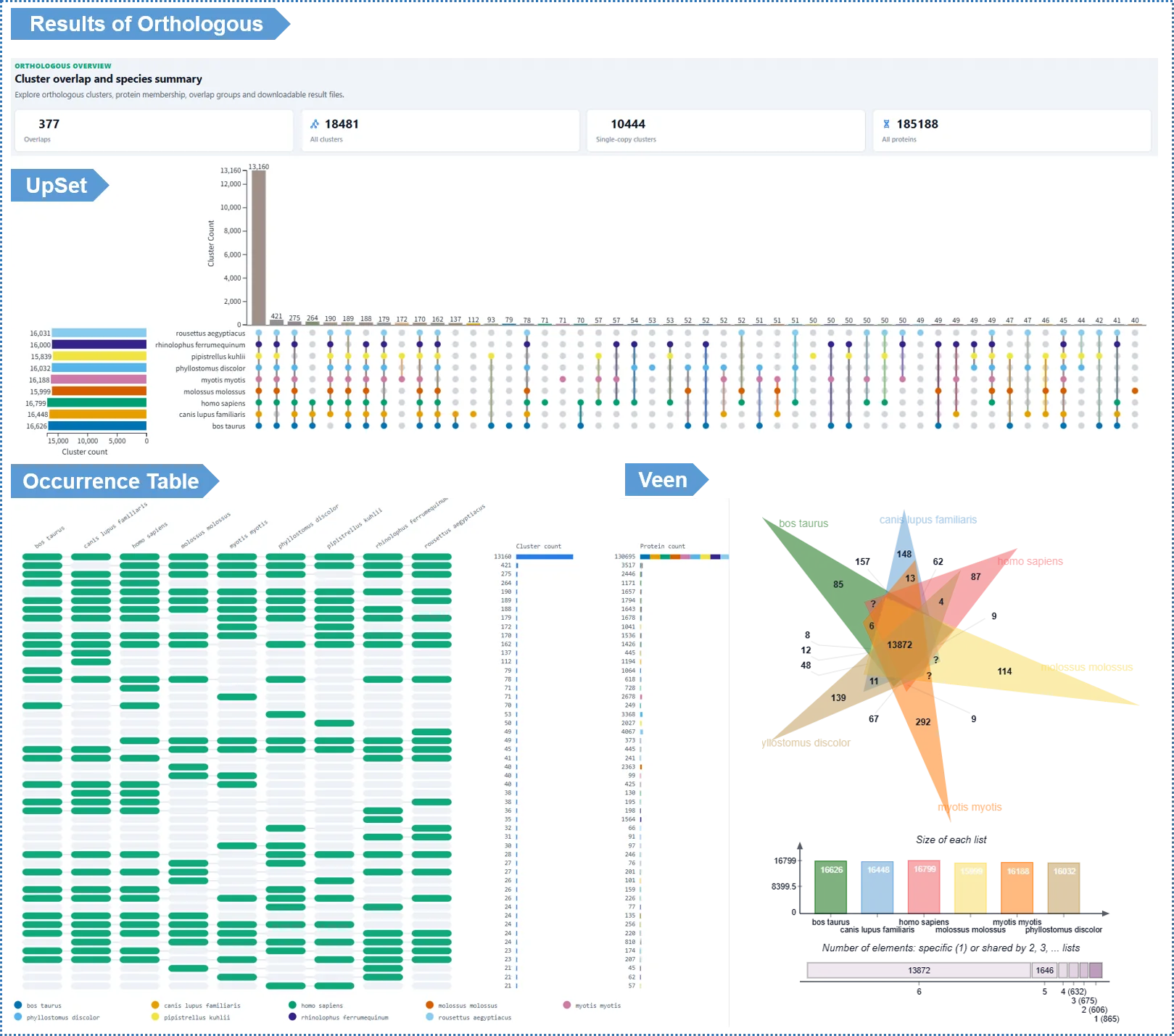
- UpSet plot: shows the distribution of clusters shared and unique among species; click an intersection bar to see the specific clusters in that intersection.
- Venn diagram: the classic Venn (suitable for ≤6 species).
- Pairwise shared-cluster heatmap: a matrix showing, for every species pair, the number of clusters they share — a quick read on overall similarity among species.
- Occurrence Table: a matrix showing each cluster's copy number in every species; sort by column to find clusters with a specific distribution pattern.
- Pan-genome statistics: total proteins, cluster count, single-copy gene count and singleton count for each species.
- Single-cluster detail: click any cluster ID to see species composition, multiple sequence alignment, conserved motifs, the within-cluster gene tree, the similarity network, cluster-to-cluster relationships, and GO enrichment — this is also where you launch positive selection analysis (see Chapter 9).
Quick glossary (cluster categories):
| Term | Meaning |
|---|---|
| Orthogroup / Cluster | A set of homologous genes judged to descend from a common ancestral gene |
| 1:1:1 (single-copy core cluster) | An orthologous cluster withexactly one copy in every species — the ideal data for building a species tree |
| N:N:N (multi-copy core cluster) | A cluster containingall species but with multiple copies in at least some of them |
| Species-specific cluster | A cluster whose genes areall from one species, often related to that species' unique functions |
| Other / Orthoer cluster | A (multi-copy) orthologous cluster containing onlysome of the species |
| Singletons | Isolated genesnot assigned to any cluster (no homology found) |
| Core genome | The set of clusters shared by all species |
| Pan-genome | The union of all clusters across all species |
| Ortholog vs paralog | Orthologs arise fromspeciation; paralogs arise from gene duplication |
5.2 Module 2 · Species Tree Analysis
What does this module do for you? It builds a species phylogeny from the single-copy orthologs of Module 1. This tree is the "evolutionary scaffold" for downstream analyses such as divergence time, gene family dynamics and positive selection.
How to enable: tick Species Tree on the left.
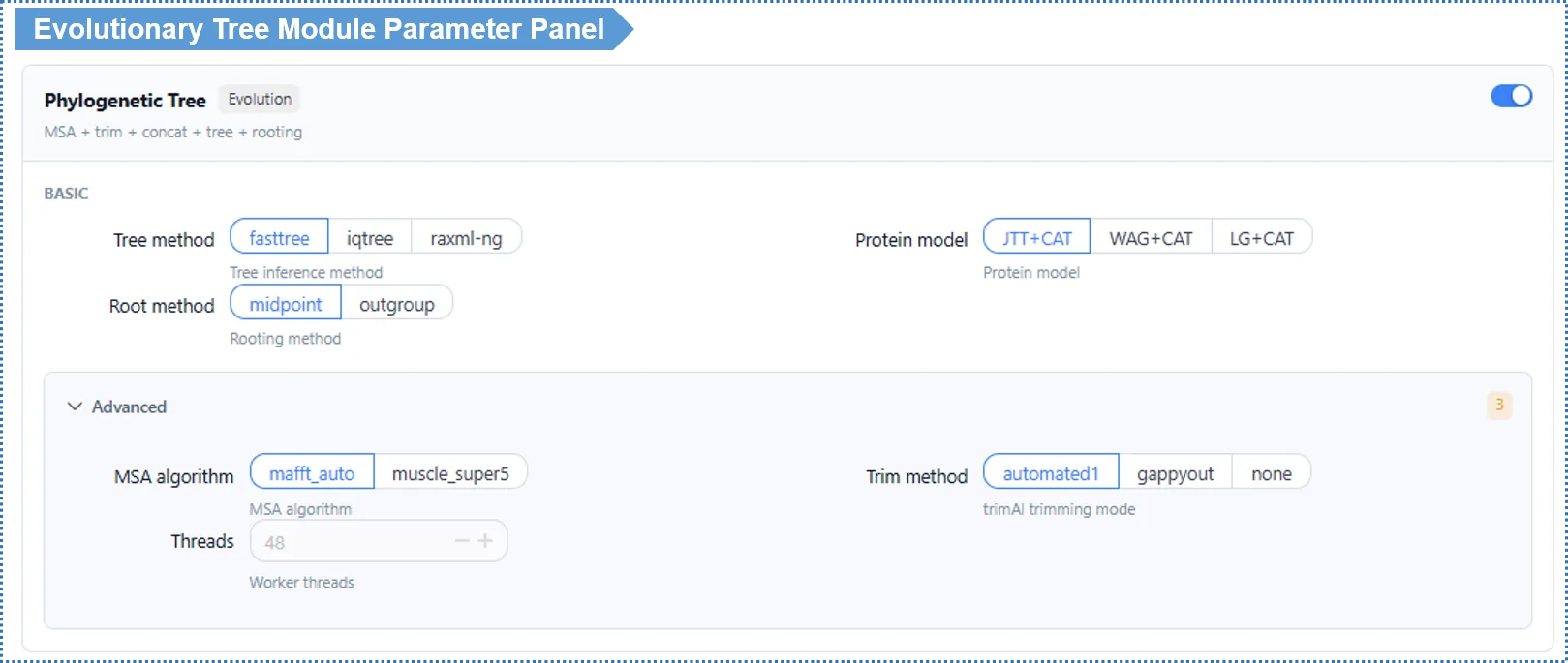
Basic Parameters
Tree method — default FastTree
| Method | Speed | Accuracy | Use case |
|---|---|---|---|
| FastTree (default) | Fastest (minutes) | Good | Online analysis, quick preview, many species |
| IQ-TREE 2 | Slower (tens of minutes up) | High | When you want publication-grade accuracy; built-in ModelFinder selects the model automatically |
| RAxML-NG | Slower | High | A strict maximum-likelihood method, comparable to IQ-TREE 2; good for cross-validating topology with a different method |
How to choose? For online analysis we recommend FastTree — fast and good enough for most studies. If you need publication-grade accuracy and can accept a longer wait, choose IQ-TREE 2 (with automatic model selection); to cross-validate your tree with another mainstream maximum-likelihood implementation, use RAxML-NG. For large-scale analyses, use the local deployment.
Root method — default Midpoint
| Method | Meaning | Use case |
|---|---|---|
| Midpoint (default) | Places the root at the midpoint of the longest path | Quick and convenient when the outgroup is uncertain |
| Outgroup | Designates a known outgroup species as the root | More reliable when a clear outgroup exists |
When you choose Outgroup, an outgroup species selector appears below. The outgroup should be a species clearly related to all study species but lying outside the study group (e.g. grape Vitis vinifera as the outgroup when studying Rosaceae).
Advanced Parameters
| Parameter | Default | Description |
|---|---|---|
| MSA algorithm | MAFFT Auto | MUSCLE v5 Super5 available for large data |
| Substitution model | Auto-detect (MFP) / LG+CAT | See note below |
| Alignment trimming | automated1 | gappyout / none available (none for experts only) |
| Threads | 48 | Read-only online; editable locally |
About substitution models and auto-detection (MFP): the substitution model describes the frequency and pattern of amino-acid substitutions during evolution; choosing wrongly can produce an incorrect topology.
- With IQ-TREE 2 / RAxML-NG, the default is MFP (ModelFinder Plus) auto-detection: the algorithm uses information criteria (BIC / AIC) to pick the best-fitting model from a set of candidates automatically, with no manual specification needed. If you already know a suitable model, you can fill it in manually to skip detection time.
- With FastTree, a fixed LG+CAT model is used (WAG / JTT also selectable); no model search is performed, which is why it is faster.
Interpreting the Results
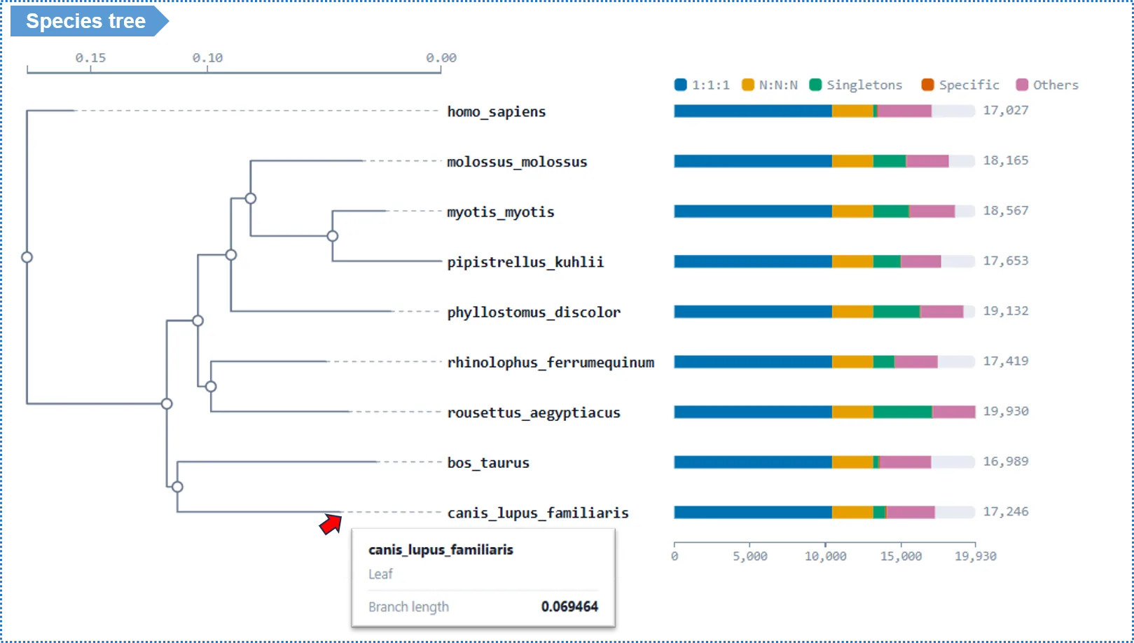
- Hover over a tree node to see its bootstrap support: ≥95% highly reliable, 70%–95% moderate, <70% interpret with caution.
- The tree can be exported as Newick text and as SVG / PNG images.
Quick glossary:
| Term | Meaning |
|---|---|
| Topology | The branching structure of the tree, i.e. who is more closely related to whom |
| Bootstrap support | A percentage assessing the reliability of a branch via resampling; higher is more reliable |
| Newick | The standard text format using nested parentheses to represent a tree |
| Single-copy orthologs | The 1:1:1 clusters from Module 1, used as input for tree building |
5.3 Module 3 · Divergence Time Estimation
What does this module do for you? It converts the "relative" tree from Module 2 into a "time tree" labeled with absolute geological ages. Using fossil calibration points and a molecular-clock model, it estimates the divergence time of each node, letting you map genome-evolution events onto geological and climatic events.
How to enable: tick Time Tree (depends on Module 2).
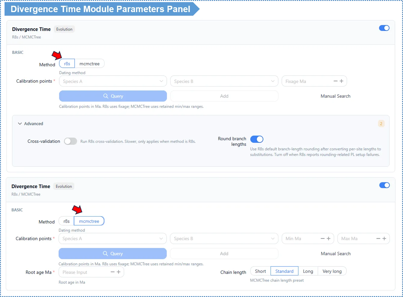
Basic Parameters
Method — default R8s
| Method | Speed | Output | Use case |
|---|---|---|---|
| R8s (default) | Fast (minutes) | Point estimates of node ages | A quick divergence-time framework |
| MCMCTree | Slower (tens of minutes up) | Times + 95% HPDconfidence intervals | Publication-grade; when uncertainty intervals are needed |
How to choose? For a quick sense of divergence times, use R8s. For publication, when you need a 95% confidence interval per node, use MCMCTree (slower; large-scale analyses are best run locally).
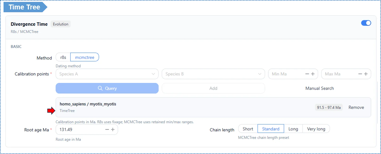
Calibration points — required; this is the most critical input of this module
- Pick a species pair, and the platform can automatically look up their divergence time from the TimeTree database. Click + to add multiple sets; at least 1–2 are recommended.
- The two methods use the calibration information differently:
- R8s uses the median divergence time returned by TimeTree (a single point). R8s does not propagate calibration uncertainty and only gives point estimates, so using the median is more stable and more honest.
- MCMCTree uses the range returned by TimeTree (minimum / maximum) and performs Bayesian sampling within that interval, yielding a 95% HPD confidence interval.
- Source guidance: prefer field-recognized calibration points backed by paleontological/geological evidence. An incorrect calibration point will systematically bias the entire time tree.
Example settings (Rosaceae):
| Species pair | Min (Ma) | Max (Ma) | Basis |
|---|---|---|---|
| Malus domestica – Pyrus communis | 12 | 20 | Fossil record |
| Malus domestica – Vitis vinifera | 110 | 124 | Fossil record |
Root Age (Ma)
- Default: the platform automatically sets it to 1.5× the largest branch divergence time in the current tree.
- ⚠️ We strongly recommend confirming this value manually. Root Age is the global constraint on divergence times for the whole tree; it must be greater than the true divergence time of the oldest (root) node, otherwise the entire time tree is compressed and you get incorrect age estimates.
- If you are unsure of the exact value, err on the high side — it serves only as an upper-bound constraint, so being too high does not distort results substantially, whereas being too low certainly causes errors. You can consult TimeTree (https://timetree.org) for an approximate root age for your group.
Advanced Parameters
| Parameter | Default | Description |
|---|---|---|
| Cross-validation (R8s) | Off | Slower when on |
| Chain length / computational complexity (MCMCTree only) | Standard | Increase when intervals are too wide or repeated runs differ markedly, to ensure MCMC convergence |
| Threads | 48 | Read-only online; editable locally |
Interpreting the Results
- Time tree: an ultrametric tree with the horizontal axis as geological time (millions of years ago); MCMCTree additionally gives a 95% HPD interval for each node.
Quick glossary:
| Term | Meaning |
|---|---|
| Ultrametric tree | A tree in which all leaves are equidistant from the root, i.e. branch lengths converted to time |
| Ma / Mya | Time units; 1 Ma = 1 million years |
| Molecular clock | The modeling assumption that uses the rate of sequence change to infer time |
| 95% HPD interval | Highest posterior density interval, the divergence-time confidence range from a Bayesian method (MCMCTree) |
| Calibration point | A known divergence time of a species pair, used to anchor the relative tree to absolute ages |
5.4 Module 4 · Gene Family Expansion & Contraction Analysis
What does this module do for you? Using the time tree from Module 3 and the gene counts from Module 1, it identifies gene families that underwent statistically significant expansion (gene gain) or contraction (gene loss) on each branch of the species tree. Such changes are often linked to adaptive evolution, functional innovation or degeneration — for example, a significant expansion of a disease-resistance gene family on a cultivated lineage may point to selection during domestication.
How to enable: tick Gene Family Expansion & Contraction (depends on Modules 1 and 3). The algorithm is CAFE5 (based on a stochastic birth-death model).
Basic Parameters
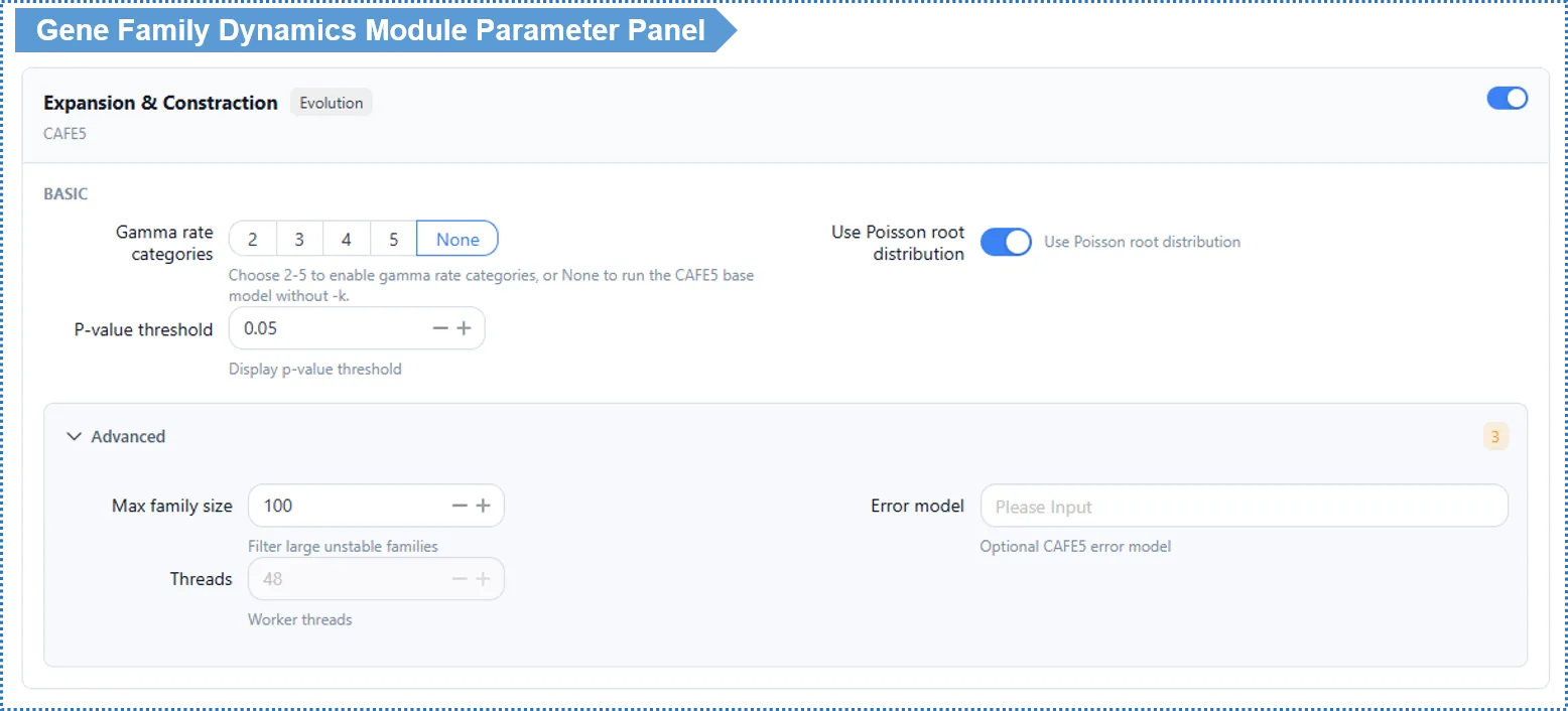
k value (rate heterogeneity among gene families) — determines whether the Base model or the Gamma model is used
| Setting | Model used | Meaning | When to use |
|---|---|---|---|
| k left empty (none) | Base model | Assumes all gene families share exactly the same evolutionary rate (λ) | Small data, first pass; or for a robust analysis whose failures are easy to detect |
| k = 2 | Gamma model | Allows family rates to follow a 2-category gamma distribution | A common choice in most scenarios |
| k = 3 or more | Gamma model | More rate categories, finer fit | Large data, pronounced rate differences among families |
How it works: the Gamma model (allowing different families to evolve at different rates) is enabled only when a k value is set; leaving k empty uses the Base model (a single rate).
How to choose? In real data, different families almost certainly evolve at different rates (immune genes fast, ribosomal proteins slow), so a k=2 Gamma model is usually more reasonable than Base — we suggest starting from k=2. However, the Gamma model can fail silently when it does not converge, whereas problems with the Base model are easier to spot — so if you want the most robust, diagnosable baseline, run Base (k empty) once for comparison first.
Convergence safeguards for the Gamma model: because the Gamma model can fail silently, when you set a k value the platform automatically runs multiple restarts and reports the convergence quality of the run. Inspect this convergence report before trusting a Gamma result; if convergence is poor, prefer the Base model or adjust the parameters.
Use Poisson root distribution (Use Poisson) — default on, recommended to keep.
Advanced Parameters
| Parameter | Default | Description |
|---|---|---|
| Max family size | 100 | Filters out very large families to avoid non-convergence |
| Error model | None | Optional (expert); when empty, the platform automatically downgrades and retries |
| Threads | 48 | Read-only online; editable locally |
Significance threshold (p-value, default 0.05): used to decide which families have a statistically significant size change on a given branch. This threshold also determines the family set used for the subsequent GO enrichment analysis (see results). Adjusting it on the results page only refreshes the view and does not rerun the analysis; set 0.01 for stricter, 0.10 to see more candidate families.
Interpreting the Results
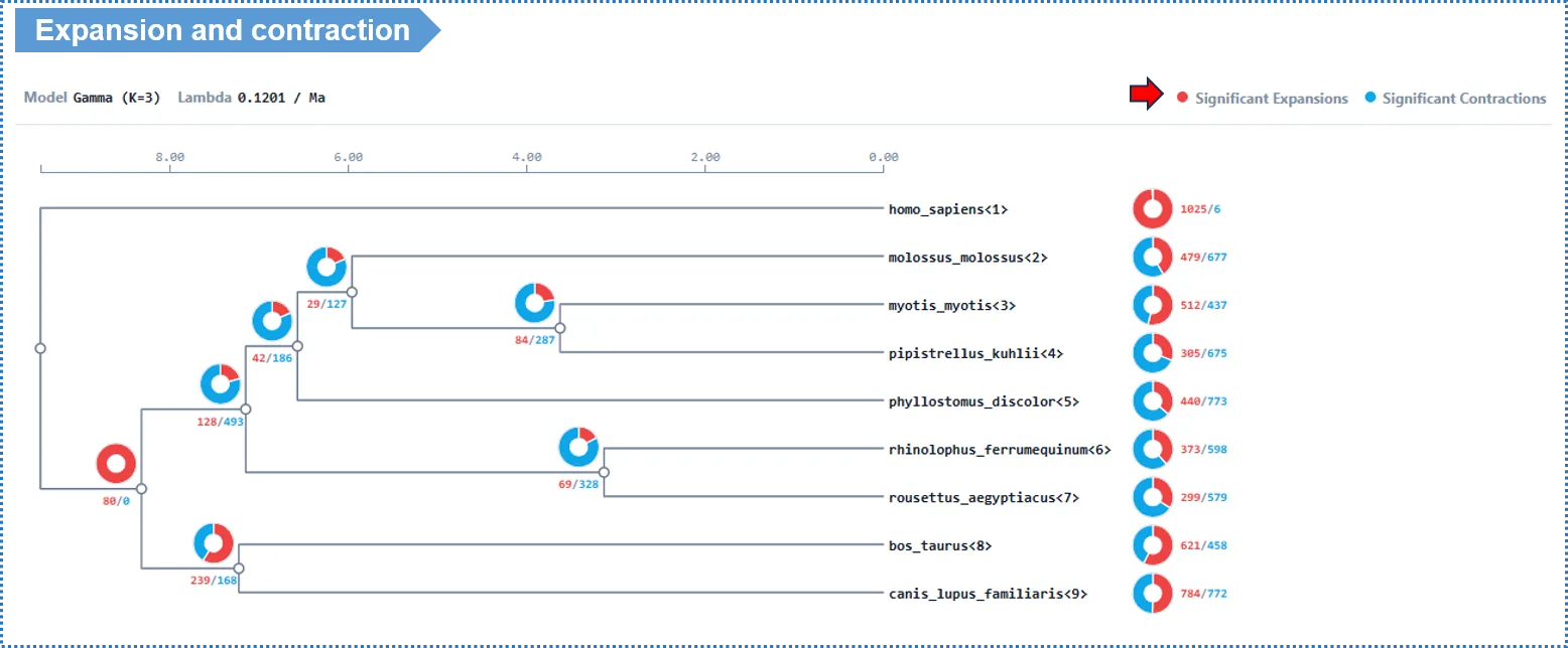
- Each branch of the species tree is labeled with two numbers: a red + for the number of families that expanded on that branch, and a blue − for the number that contracted. Note these are descriptive counts (all families with a size change on that branch), not limited to the statistically significant ones.
- Click the number on a branch → view the list of families that changed on that branch; click a family ID → view its per-species copy number, member genes and GO annotation.
- GO enrichment: when you click an expansion/contraction node to view its GO enrichment, the platform runs enrichment only on the significant families (OG clusters) with p < 0.05 at that node, to ensure the enrichment reflects genuinely significant evolutionary events.
- It is worth focusing on the families that expanded on the terminal branch leading to your target species, to see whether their functions relate to known phenotypes.
Quick glossary:
| Term | Meaning |
|---|---|
| Expansion / Contraction | An increase / decrease in the copy number of a gene family on a branch |
| Birth-death model | The statistical model CAFE5 uses to describe gene gain (birth) and loss (death) |
| λ (lambda) | The gene gain/loss rate; one λ across the whole tree in the Base model, family-specific in the Gamma model |
| Base vs Gamma model | See the Basic-parameter note on k: empty k uses Base, set k uses Gamma |
| Significant family | A family with p < 0.05; GO enrichment uses only these |
5.5 Module 5 · Chromosomal Collinearity Analysis
What does this module do for you? It analyzes structural conservation between species at the chromosomal level. If certain chromosomal segments of two species contain the same genes in roughly the same order, those segments are said to be "collinear". This can reveal: the degree of chromosomal-structure conservation, large-scale rearrangements (inversions/translocations/fusions/fissions), traces of whole-genome duplication (WGD), and the chromosomal distribution of particular gene families.
Data requirement: upload a GFF annotation file (see 2.5).
⚠️ Be sure to use a chromosome-level annotation file, and keep the number of distinct chromosomes below 50. Collinearity analysis uses chromosomes as coordinate axes, and too many sequence fragments make the Sankey diagram unreadable.
- If your annotation is at the scaffold / contig level (many fragments), filter first and keep only the 50 longest fragments before uploading.
- Chromosome-level genomes (e.g. a reference genome already anchored to chromosomes) can be used directly.
How to enable: tick Collinearity / MCScanX.
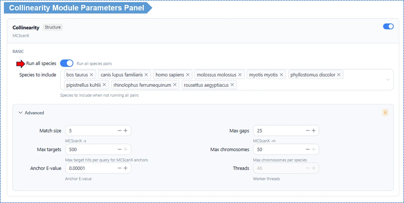
Basic Parameters
Run all species pairs (Run All Pairs) — default on (small projects)
- On: runs collinearity for every species pair. Recommended when there are few species.
- Off: a species-pair selector appears so you run only the pairs you choose. Recommended when there are many species, to save time.
Advanced Parameters
| Parameter | Default | Description |
|---|---|---|
| Match Size (-s) | 5 | Minimum number of anchor genes in a collinear block |
| Max Gaps (-m) | 25 | Maximum gap allowed within a block |
| Anchor E-value (-e) | 1e-5 | Anchor alignment threshold |
| Threads | 48 | Read-only online; editable locally |
The up/down-stream gene window is adjusted on the results page and only refreshes the view.
Interpreting the Results
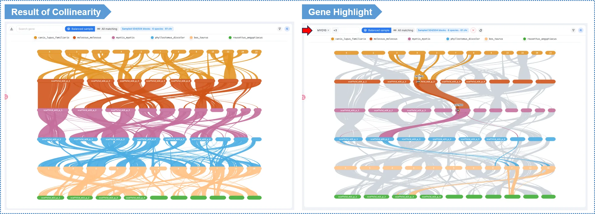
- Sankey diagram: the two sides represent the chromosomes of two species, and the links are collinear blocks; denser links mean more conserved structure, while breaks and crossings represent rearrangement events.
- Gene-search highlighting (signature feature): type a gene ID in the search box (e.g. a member of an expanded family found in Module 4), and the plot highlights the collinear blocks containing those genes — linking gene-family dynamics to chromosomal-structure change.
Quick glossary:
| Term | Meaning |
|---|---|
| Collinearity / Synteny | Chromosomal segments of two species containing the same genes in roughly the same order |
| Collinear block | A region of consecutive homologous genes judged to be conserved |
| Anchor | A pair of homologous genes within a block; the basis for the collinearity call |
| Sankey diagram | A plot using links to show collinear relationships between the chromosomes of two species |
| Rearrangement | Chromosomal structural changes such as inversion, translocation, fusion, fission |
| WGD (whole-genome duplication) | Leaves traces of doubled blocks in collinearity |
6. Step 3: Preview & Submit
- Once the desired modules are configured, click Preview to review a summary of the task configuration.
- After confirming everything is correct, click Submit.
- The page shows a unique Task ID — save it so you can check progress.
- The task runs in the background, so you may close the browser; on completion the system sends an email with a link to the results page.
Tip: keep your Task ID. Provide a valid email if you want the completion notification.
7. Tracking Progress & Task History
- Click Projects / Task History to see all tasks and their status (queued / running / completed / failed).
- Click a Task ID to open its results page.
8. Interpreting & Exporting Results
8.1 Interactive Exploration
All results are interactive visualizations. You can: click elements in a plot (clusters, tree nodes, Sankey blocks) to see details; hover to see exact values (support, divergence time, p-value); filter and sort tables; search gene IDs; and zoom and drag plots.
8.2 Export
- Graphics: all charts can be exported as SVG (vector, publication-ready) or PNG.
- Data: cluster lists, Newick tree files, statistics tables (TSV / CSV), etc. can be downloaded.
- BLAST database: the project also provides a pre-built BLAST database of all project proteins for download, so you can run your own sequence searches locally.
- Cloud: one-click export to Google Drive or Dropbox.
8.3 Analysis Report (Reproducibility)
Each analysis automatically generates a report recording the parameters used, the versions of the integrated tools, and the full command history, so others can independently reproduce it with the same data and parameters.
9. Positive Selection Analysis on Gene Clusters (run on demand after results are generated)
What does this analysis do for you? It detects which genes underwent positive selection (adaptive evolution). The molecular signal is a non-synonymous substitution rate significantly higher than the synonymous rate, i.e. ω = dN/dS > 1 — meaning natural selection "favors" mutations that change protein function, often associated with adaptation to a new environment.
It differs from the first five modules: positive selection targets a single gene cluster, requiring you to first see the results and then pick a cluster of interest (e.g. a significantly expanded family, a cluster with significant GO enrichment). It is therefore not in the submission wizard but triggered on demand on the results page.
9.1 Prepare CDS
This analysis requires the species' CDS nucleotide sequences (see 2.4). If you did not upload CDS when adding the species, you can add CDS to the species data at any time — adding it later unlocks only positive selection and does not affect results already completed. Built-in database species already have CDS ready.
9.2 Entry Point
On the cluster detail page, click "Positive Selection Analysis", or launch it directly from result highlights (CAFE5 significant families, GO-enriched clusters, search-hit clusters).
9.3 Choose Your Scientific Question (key)
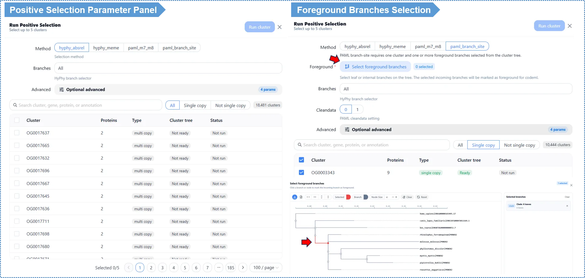
The top of the dialog asks: What do you want to find out about this cluster? You do not need to understand the internal differences between tools — just choose the question you want to answer; the algorithm name is shown as a subtitle.
| The question you want to answer (interface text) | Method | Output granularity | Extra input needed |
|---|---|---|---|
| Which branches (lineages) show positive selection? | HyPhy aBSREL (recommended, default) | Branch level | No |
| Which amino-acid sites show episodic positive selection? | HyPhy MEME | Site level | No |
| Does this family contain any positively selected sites? | PAML M7 vs M8 (expert) | Site level | No |
| On branches I select, which sites are under positive selection? | PAML branch-site (expert) | Site level | Foreground branches must be selected on the tree |
Unsure which to choose? Start with aBSREL — the fastest and most robust, ideal for a first analysis. To pinpoint specific amino-acid sites, use MEME (when you suspect episodic selection on only some branches) or PAML M7/M8 (to detect persistent positively selected sites across the whole tree). If you already have a hypothesis that a lineage is under selection, use PAML branch-site and mark the foreground branches on the tree.
9.4 Other Options
- Foreground branches (branch-site only): an interactive cluster tree pops up; click the species or lineages you hypothesize to be under selection; at least 1 must be selected to submit.
- Genetic code (Advanced): defaults to the Universal code; species with non-standard codes (mitochondria, ciliates, etc.) need to switch here.
- Threads (Advanced): read-only 48 online; editable locally.
- Online size limit: online analysis allows at most 100 proteins per cluster. For larger clusters, pick a smaller one or use the local deployment (see Chapter 11).
- The first time you analyze a cluster, the platform builds its alignment and tree (once only), so please wait a moment.
9.5 Interpreting the Results
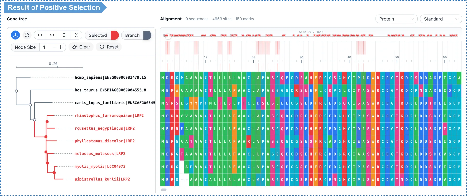
| Method | Result display | Filters adjustable on the results page |
|---|---|---|
| aBSREL | Branch-level table + tree (significant branches highlighted) | p-value |
| MEME | Site-level table + alignment (significant sites highlighted) | p-value, EBF |
| PAML M7/M8 | Site-level table (likelihood-ratio test + posterior) | p-value, BEB posterior |
| PAML branch-site | Site-level table on the foreground branches | p-value, BEB posterior |
- Amino-acid sites identified as positively selected by the Bayesian methods (BEB / EBF) are highlighted (e.g.
128 A*) — these are the specific positions that bear an adaptive signature at the molecular level. - Adjusting the thresholds on the results page only refreshes the view and does not rerun the analysis.
Quick glossary:
| Term | Meaning |
|---|---|
| dN/dS (ω) | The ratio of non-synonymous to synonymous substitution rates; ω > 1 suggests positive selection |
| Positive selection | Natural selection favoring mutations that change protein function, i.e. adaptive evolution |
| Branch level vs site level | Branch level answers "which lineages are under selection"; site level answers "which amino-acid sites are under selection" |
| Foreground branch | In branch-site, the branch you hypothesize to be under selection and must mark on the tree |
| Episodic selection | Positive selection occurring on only some branches or at only some times |
| BEB / EBF | Bayesian empirical methods giving the posterior probability / empirical Bayes factor that a site is under positive selection |
Different methods detect different types of selection signal; we recommend trying several methods on the same cluster to obtain complementary evidence.
10. Online Helper Tools (Web Tools)
The TOOLS menu provides three standalone tools you can use without submitting a task.
10.1 Cluster-Venn: General-Purpose Orthologous-Cluster Venn Diagram
Upload a custom cluster-membership file to directly generate an interactive Venn / UpSet plot, with no need to re-run clustering on the platform. Ideal when you have already clustered with a third-party tool (OrthoFinder, OrthoMCL, etc.) and just want a quick visualization.
Input format (.csv / .txt): one cluster per line, genes within a cluster separated by spaces, gene names in the form SpeciesName|GeneID; the platform identifies species membership by the prefix before |.
SpeciesA|bin1 SpeciesA|bin2 SpeciesB|fin1 SpeciesB|fin2 SpeciesC|gin2
SpeciesA|bin22 SpeciesB|fin22 SpeciesC|gin24
SpeciesB|fin32 SpeciesC|gin624
10.2 GFF to BED: Annotation Format Conversion
Converts a standard 9-column GFF / GFF3 into a 4-column / 5-column BED that meets the input requirements of collinearity analysis. GFF3 downloaded from Ensembl / NCBI / Phytozome can be converted in one click and then uploaded.
10.3 Newick Viewer: Online Phylogenetic Tree Viewer
Upload or paste a Newick tree file to view and interactively browse its topology online. Handy for quickly checking that a tree file is correct and previewing its shape.
11. Local Deployment (Docker)
For users with higher demands on analysis scale, compute speed or data privacy.
- No limit on species count: the online version limits concurrent analysis to 12 species to keep shared resources fair; the local version removes this limit, enabling large-scale comparisons of dozens of species.
- Uses local compute, faster: tasks run locally with no queue; computation on large datasets is significantly faster.
- Customizable thread count: the thread-count parameter in each module's Advanced section is editable in the local version, so you can fully use a multi-core CPU (fixed at 48 and non-editable online).
- Larger positive-selection scale: the per-cluster protein cap can be raised (limited to 100 online).
- Data privacy / offline: data is processed entirely locally, suitable for unpublished or sensitive data; once deployed, it can run offline.
How to deploy: distributed as a Docker container; installation and configuration are on the DOWNLOAD page of the homepage.
12. FAQ & Troubleshooting
| Problem | Possible cause | Solution |
|---|---|---|
| Upload fails or reports a format error | Special characters in FASTA headers; GFF/CDS IDs do not match the protein | Preprocess and validate ID consistency with the online helper tools (Chapter 10) |
| Task stays "queued" for a long time | High load on the public server | Wait for the email notification; for more speed, use the Docker local version |
| Species-tree topology disagrees with known relationships | Too few single-copy genes (<50); or insufficient method accuracy | Check the number of single-copy genes; switch to IQ-TREE 2 for higher accuracy |
| Divergence-time intervals too wide or results unstable | Insufficient calibration points; MCMC did not converge | Add reliable calibration points; increase chain length / complexity in MCMCTree |
| No significant positive-selection signal | Too few substitution events; weak signal | Switch to aBSREL to detect episodic selection; look at genes with elevated but non-significant ω |
| Positive selection reports protein count over the limit | The cluster has >100 proteins (online cap) | Choose a smaller cluster, or analyze large families with the local version |
| CDS / GFF reports a mismatch after upload | IDs do not match the protein file | Ensure IDs are exactly identical; validate with the online tool (see 2.2) |
| Collinearity plot is very sparse | Species are too distant; GFF is incomplete | Compare more closely related species pairs; check gene coverage of the GFF |
Getting help: for questions, contact us via the homepage, or see the DOCUMENTATION page.
Citing OrthoVenn: if you use OrthoVenn in your research, please cite the corresponding paper (refer to the latest release on the platform homepage).